Creating a Four-step Transportation Model in Python
A four-step transportation model predicts the traffic load on a network given data about a region. These models are used to evaluate the impacts of land-use and transportation projects. In this example, we will create a model representing California as if it acted as a city. To get started, first we will import the necessary libraries. All of these can be installed from pip.
import requests
import pandas
import geopandas
import json
import math
from haversine import haversine
from ipfn import ipfn
import networkx
from matplotlib import pyplot
from matplotlib import patheffects
Step 0 Gather Data
First we need some data about the study area. Supply data is the transportation network including roads, public transportation schedules, etc. To keep things simple, we are going to assume the transport network is a line connecting the centroid of each zone to the centroid of each other zone.
Supply Data
url = 'https://tigerweb.geo.census.gov/arcgis/rest/services/TIGERweb/State_County/MapServer/37/query?where=state%3D06&f=geojson'
r = requests.get(url)
zones = geopandas.GeoDataFrame.from_features(r.json()['features'])
centroidFunction = lambda row: (row['geometry'].centroid.y, row['geometry'].centroid.x)
zones['centroid'] = zones.apply(centroidFunction, axis=1)
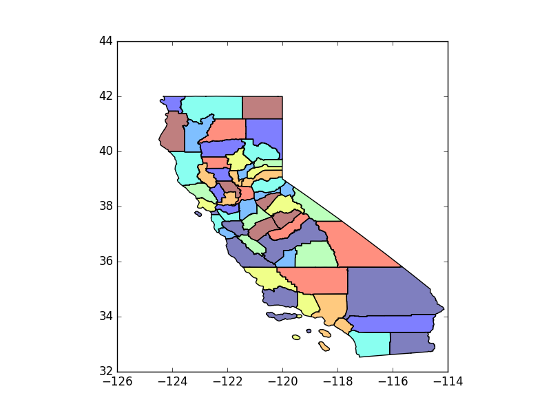
At this point we can plot our zones and see how they look:
zones.plot()
pyplot.show()
Demand Data
Demand dats is the users of the transportation network. For passenger models, demand data is typically census data including residential locations, work locations, school location, etc. For freight models, demand data could be tons of freight, number of bananas, etc. In this case we will study workers' home locations (from the 2015 American Community Survey (ACS) 5-Year Data) and employees' locations (from the Bureau of Labor Statistics (BLS)). (The BLS API seems to be quite slow...)
url = 'http://api.census.gov/data/2015/acs5/profile?get=NAME,DP03_0018E&for=county&in=state:06'
r = requests.get(url)
Production = pandas.DataFrame(r.json()[1:], columns = r.json()[0], dtype='int')
nameSplit = lambda x: x.split(',')[0]
Production['NAME'] = Production['NAME'].apply(nameSplit)
zones = pandas.merge(zones, Production)
zones['Production'] = zones['DP03_0018E']

def getEmployment(state, county):
  prefix = 'EN'
  seasonal_adjustment = 'U'
  area = format(state, "02d") + format(county, "03d")
  data_type = '1'
  size = '0'
  ownership = '0'
  industry = '10'
  seriesid = prefix + seasonal_adjustment + area + data_type + size + ownership + industry
  headers = {'Content-type': 'application/json'}
  data = json.dumps({"seriesid": [seriesid],"startyear":"2015", "endyear":"2015", "registrationKey": ""})
  p = requests.post('https://api.bls.gov/publicAPI/v2/timeseries/data/', data=data, headers=headers)
  employment = p.json()['Results']['series'][0]['data'][0]['value']
  return(employment)

employment = lambda row: int(getEmployment(row['state'], row['county']))
zones['Attraction'] = zones.transpose().apply(employment)
zones['Production'] = zones['Production'] * zones.sum()['Attraction'] / zones.sum()['Production']
zones.index = zones.NAME
zones.sort_index(inplace=True)
The second to last line makes sure the sums of Production and Attraction are equal. Iterative Proportional Fitting in Trip Distribution will fail if they are not. We assume people with multiple jobs are spread thoughout the study area. Now let's take a look at where our commuters live and work:
pandas.set_option('display.float_format', lambda x: '%.0f' % x)
zones[['Production', 'Attraction']].head()
| Production | Attraction | |
|---|---|---|
| Alameda County | 691588 | 741843 |
| Alpine County | 380 | 531 |
| Amador County | 11425 | 11500 |
| Butte County | 83232 | 79361 |
| Calaveras County | 15044 | 8888 |
We can easily see that Alameda and Alpine Counties see an influx of commuters during the day and Butte and Calaveras Counties are the opposite.
Step 1 Trip Generation
Trip Generation is where we compute the numbers for Production and Attraction. We completed this above.
Step 2 Trip Distribution
In Trip Distribution we use a Gravity Model to calculate a cost matrix representing the cost of travel between each pair of zones. First, we create a simple cost function. Then we use that function to calculate our cost matrix by interating through all possible zone pairs. Then we can use our cost matrix to distribute our trips across our study area. Changing the beta parameter adjusts the Friction of Distance. Beta will vary based on the units of distance. We use a Haversine Function to calculate distances in kilometers (or miles) from geographic coordinates. The Trip Distribution function uses Iterative Proportional Fitting to assign trips from our Production and Attraction arrays to our matrix.
def costFunction(zones, zone1, zone2, beta):
  cost = math.exp(-beta * haversine(zones[zone1]['centroid'], zones[zone2]['centroid']))
  return(cost)

def costMatrixGenerator(zones, costFunction, beta):
  originList = []
  for originZone in zones:
    destinationList = []
    for destinationZone in zones:
        destinationList.append(costFunction(zones, originZone, destinationZone, beta))
    originList.append(destinationList)
  return(pandas.DataFrame(originList, index=zones.columns, columns=zones.columns))

def tripDistribution(tripGeneration, costMatrix):
  costMatrix['ozone'] = costMatrix.columns
  costMatrix = costMatrix.melt(id_vars=['ozone'])
  costMatrix.columns = ['ozone', 'dzone', 'total']
  production = tripGeneration['Production']
  production.index.name = 'ozone'
  attraction = tripGeneration['Attraction']
  attraction.index.name = 'dzone'
  aggregates = [production, attraction]
  dimensions = [['ozone'], ['dzone']]
  IPF = ipfn.ipfn(costMatrix, aggregates, dimensions)
  trips = IPF.iteration()
  return(trips.pivot(index='ozone', columns='dzone', values='total'))

beta = 0.01
costMatrix = costMatrixGenerator(zones.transpose(), costFunction, beta)
trips = tripDistribution(zones, costMatrix)
If we take a look at the trips table we can see that most trips stay inside each county, but some go quite far. Origin zones are on the left. Destination zones are on the top.
| Alameda County | Alpine County | Amador County | Butte County | Calaveras County | Colusa County | Contra Costa County | Del Norte County | El Dorado County | Fresno County | Glenn County | Humboldt County | Imperial County | Inyo County | Kern County | Kings County | Lake County | Lassen County | Los Angeles County | Madera County | Marin County | Mariposa County | Mendocino County | Merced County | Modoc County | Mono County | Monterey County | Napa County | Nevada County | Orange County | Placer County | Plumas County | Riverside County | Sacramento County | San Benito County | San Bernardino County | San Diego County | San Francisco County | San Joaquin County | San Luis Obispo County | San Mateo County | Santa Barbara County | Santa Clara County | Santa Cruz County | Shasta County | Sierra County | Siskiyou County | Solano County | Sonoma County | Stanislaus County | Sutter County | Tehama County | Trinity County | Tulare County | Tuolumne County | Ventura County | Yolo County | Yuba County | |
|---|---|---|---|---|---|---|---|---|---|---|---|---|---|---|---|---|---|---|---|---|---|---|---|---|---|---|---|---|---|---|---|---|---|---|---|---|---|---|---|---|---|---|---|---|---|---|---|---|---|---|---|---|---|---|---|---|---|---|
| Alameda County | 128707 | 17 | 667 | 6631 | 487 | 853 | 53313 | 352 | 2785 | 6306 | 794 | 2225 | 8 | 12 | 1046 | 866 | 1392 | 540 | 4519 | 1066 | 11156 | 146 | 2261 | 4466 | 128 | 87 | 14127 | 8389 | 1818 | 1032 | 8716 | 343 | 96 | 56378 | 1188 | 151 | 336 | 70696 | 21329 | 3870 | 50131 | 3160 | 131790 | 13520 | 4663 | 26 | 820 | 17628 | 17322 | 13558 | 2803 | 1417 | 179 | 829 | 571 | 1412 | 11066 | 1337 |
| Alpine County | 18 | 0 | 2 | 4 | 2 | 0 | 9 | 0 | 11 | 46 | 0 | 1 | 0 | 0 | 8 | 4 | 0 | 2 | 33 | 9 | 2 | 1 | 0 | 8 | 0 | 1 | 8 | 2 | 5 | 8 | 23 | 1 | 1 | 35 | 1 | 2 | 3 | 10 | 13 | 7 | 7 | 8 | 31 | 2 | 3 | 0 | 0 | 4 | 3 | 14 | 1 | 1 | 0 | 8 | 6 | 7 | 3 | 1 |
| Amador County | 839 | 2 | 84 | 184 | 55 | 11 | 412 | 5 | 339 | 551 | 10 | 24 | 1 | 1 | 85 | 60 | 13 | 43 | 342 | 102 | 80 | 15 | 21 | 244 | 9 | 10 | 273 | 74 | 155 | 80 | 836 | 24 | 9 | 1649 | 33 | 15 | 28 | 480 | 605 | 157 | 327 | 142 | 1379 | 102 | 109 | 3 | 17 | 173 | 136 | 574 | 56 | 24 | 2 | 76 | 65 | 89 | 144 | 48 |
| Butte County | 7901 | 5 | 174 | 4781 | 115 | 220 | 4434 | 117 | 856 | 1141 | 246 | 594 | 2 | 3 | 175 | 130 | 276 | 316 | 708 | 211 | 1239 | 31 | 454 | 650 | 86 | 23 | 1150 | 1210 | 730 | 165 | 3094 | 186 | 19 | 12193 | 118 | 32 | 57 | 6729 | 3221 | 413 | 3669 | 347 | 9446 | 830 | 2749 | 11 | 421 | 2163 | 2478 | 1979 | 938 | 631 | 59 | 157 | 138 | 191 | 2204 | 610 |
| Calaveras County | 1066 | 3 | 96 | 211 | 90 | 12 | 514 | 5 | 421 | 888 | 12 | 28 | 1 | 2 | 136 | 97 | 16 | 51 | 551 | 164 | 98 | 24 | 24 | 372 | 10 | 15 | 394 | 89 | 180 | 128 | 967 | 28 | 14 | 1991 | 48 | 23 | 44 | 598 | 772 | 247 | 415 | 228 | 1818 | 134 | 125 | 3 | 19 | 212 | 165 | 797 | 66 | 28 | 3 | 121 | 102 | 144 | 173 | 55 |
Step 3 Mode Choice
At this point we have a matrix of the number of trips from each zone to each zone. Next we split those trips across the available modes, in this case walking, cycling, and driving. For this we create a Utility Function that describes the utility gained from the trip minus the utility lost due to travel time, cost, and other negative factors associated with the mode. We then use this utility function to determine the probability of taking each mode for each zone pair. Similar to Trip Distribution, we use these probabilities to compute a matrix. We can then multiply our trip matrix by the probability matrices to get the number of trips between each zone pair using a given mode.
def modeChoiceFunction(zones, zone1, zone2, modes):
  distance = haversine(zones[zone1]['centroid'], zones[zone2]['centroid'])
  probability = {}
  total = 0.0
  for mode in modes:
    total = total + math.exp(modes[mode] * distance)
  for mode in modes:
    probability[mode] = math.exp(modes[mode] * distance) / total
  return(probability)

def probabilityMatrixGenerator (zones, modeChoiceFunction, modes):
  probabilityMatrix = {}
  for mode in modes:
    originList = []
    for originZone in zones:
      destinationList = []
      for destinationZone in zones:
	  destinationList.append(modeChoiceFunction(zones, originZone, destinationZone, modes)[mode])
      originList.append(destinationList)
    probabilityMatrix[mode] = pandas.DataFrame(originList, index=zones.columns, columns=zones.columns)
  return(probabilityMatrix)

modes = {'walking': .05, 'cycling': .05, 'driving': .05}
probabilityMatrix = probabilityMatrixGenerator(zones.transpose(), modeChoiceFunction, modes)
drivingTrips = trips * probabilityMatrix['driving']
Now we can look at the number of driving trips between each zone pair.
| Alameda County | Alpine County | Amador County | Butte County | Calaveras County | Colusa County | Contra Costa County | Del Norte County | El Dorado County | Fresno County | Glenn County | Humboldt County | Imperial County | Inyo County | Kern County | Kings County | Lake County | Lassen County | Los Angeles County | Madera County | Marin County | Mariposa County | Mendocino County | Merced County | Modoc County | Mono County | Monterey County | Napa County | Nevada County | Orange County | Placer County | Plumas County | Riverside County | Sacramento County | San Benito County | San Bernardino County | San Diego County | San Francisco County | San Joaquin County | San Luis Obispo County | San Mateo County | Santa Barbara County | Santa Clara County | Santa Cruz County | Shasta County | Sierra County | Siskiyou County | Solano County | Sonoma County | Stanislaus County | Sutter County | Tehama County | Trinity County | Tulare County | Tuolumne County | Ventura County | Yolo County | Yuba County | |
|---|---|---|---|---|---|---|---|---|---|---|---|---|---|---|---|---|---|---|---|---|---|---|---|---|---|---|---|---|---|---|---|---|---|---|---|---|---|---|---|---|---|---|---|---|---|---|---|---|---|---|---|---|---|---|---|---|---|---|
| Alameda County | 42902 | 6 | 222 | 2210 | 162 | 284 | 17771 | 117 | 928 | 2102 | 265 | 742 | 3 | 4 | 349 | 289 | 464 | 180 | 1506 | 355 | 3719 | 49 | 754 | 1489 | 43 | 29 | 4709 | 2796 | 606 | 344 | 2905 | 114 | 32 | 18793 | 396 | 50 | 112 | 23565 | 7110 | 1290 | 16710 | 1053 | 43930 | 4507 | 1554 | 9 | 273 | 5876 | 5774 | 4519 | 934 | 472 | 60 | 276 | 190 | 471 | 3689 | 446 |
| Alpine County | 6 | 0 | 1 | 1 | 1 | 0 | 3 | 0 | 4 | 15 | 0 | 0 | 0 | 0 | 3 | 1 | 0 | 1 | 11 | 3 | 1 | 0 | 0 | 3 | 0 | 0 | 3 | 1 | 2 | 3 | 8 | 0 | 0 | 12 | 0 | 1 | 1 | 3 | 4 | 2 | 2 | 3 | 10 | 1 | 1 | 0 | 0 | 1 | 1 | 5 | 0 | 0 | 0 | 3 | 2 | 2 | 1 | 0 |
| Amador County | 280 | 1 | 28 | 61 | 18 | 4 | 137 | 2 | 113 | 184 | 3 | 8 | 0 | 0 | 28 | 20 | 4 | 14 | 114 | 34 | 27 | 5 | 7 | 81 | 3 | 3 | 91 | 25 | 52 | 27 | 279 | 8 | 3 | 550 | 11 | 5 | 9 | 160 | 202 | 52 | 109 | 47 | 460 | 34 | 36 | 1 | 6 | 58 | 45 | 191 | 19 | 8 | 1 | 25 | 22 | 30 | 48 | 16 |
| Butte County | 2634 | 2 | 58 | 1594 | 38 | 73 | 1478 | 39 | 285 | 380 | 82 | 198 | 1 | 1 | 58 | 43 | 92 | 105 | 236 | 70 | 413 | 10 | 151 | 217 | 29 | 8 | 383 | 403 | 243 | 55 | 1031 | 62 | 6 | 4064 | 39 | 11 | 19 | 2243 | 1074 | 138 | 1223 | 116 | 3149 | 277 | 916 | 4 | 140 | 721 | 826 | 660 | 313 | 210 | 20 | 52 | 46 | 64 | 735 | 203 |
| Calaveras County | 355 | 1 | 32 | 70 | 30 | 4 | 171 | 2 | 140 | 296 | 4 | 9 | 0 | 1 | 45 | 32 | 5 | 17 | 184 | 55 | 33 | 8 | 8 | 124 | 3 | 5 | 131 | 30 | 60 | 43 | 322 | 9 | 5 | 664 | 16 | 8 | 15 | 199 | 257 | 82 | 138 | 76 | 606 | 45 | 42 | 1 | 6 | 71 | 55 | 266 | 22 | 9 | 1 | 40 | 34 | 48 | 58 | 18 |
Step 4 Route Assignment
At this point we have a matrix of all trips from each zone to each zone by mode. We could use this information to calculate mode share percentages. However, we would also like to see how the trips look on the transportation network. For that, we create a graph to represent the network. Then we calculate the shortest path for each trip and add all the trips to the network ignoring capacity contraints. Last, we can visualize our trips and see how the traffic is distributed. The width of the line between centroids show the volume of traffic.
def routeAssignment(zones, trips):
  G = networkx.Graph()
  G.add_nodes_from(zones.columns)
  for zone1 in zones:
    for zone2 in zones:
      if zones[zone1]['geometry'].touches(zones[zone2]['geometry']):
        G.add_edge(zone1, zone2, distance = haversine(zones[zone1]['centroid'], zones[zone2]['centroid']), volume=0.0)
  for origin in trips:
    for destination in trips:
      path = networkx.shortest_path(G, origin, destination)
      for i in range(len(path) - 1):
        G[path[i]][path[i + 1]]['volume'] = G[path[i]][path[i + 1]]['volume'] + trips[zone1][zone2]
  return(G)

def visualize(G, zones):
  fig = pyplot.figure(1, figsize=(10, 10), dpi=90)
  ax = fig.add_subplot(111)
  zonesT = zones.transpose()
  zonesT.plot(ax = ax)
  for i, row in zones.transpose().iterrows():
    text = pyplot.annotate(s=row['NAME'], xy=((row['centroid'][1], row['centroid'][0])), horizontalalignment='center', fontsize=6)
    text.set_path_effects([patheffects.Stroke(linewidth=3, foreground='white'), patheffects.Normal()])
  for zone1 in G.edge:
    for zone2 in G.edge[zone1]:
      volume = G.edge[zone1][zone2]['volume']
      x = [zones[zone1]['centroid'][1], zones[zone2]['centroid'][1]]
      y = [zones[zone1]['centroid'][0], zones[zone2]['centroid'][0]]
      ax.plot(x, y, color='#444444', linewidth=volume/10000, solid_capstyle='round', zorder=1)
  pyplot.show(block=False)

G = routeAssignment(zones.transpose(), drivingTrips)
visualize(G, zones.transpose())
Here are our trips:
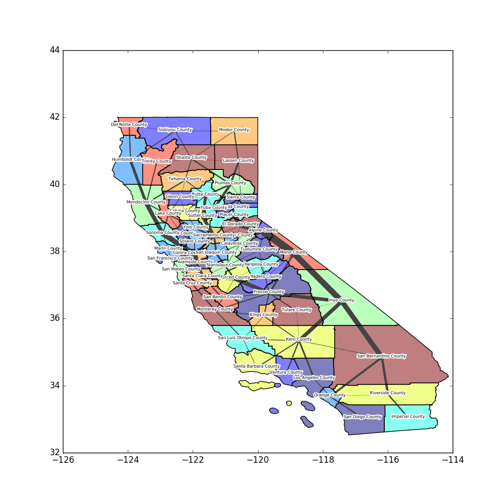
Obviously the scale of this example is quite ridiculous. Because the cost of travel is so low, our model is telling us that there will be many long distance trips. And because we used centroid-to-centroid routes, there is no concept of geography. This makes the route through the east of the state the fastest path north to south. However, this is the simple method used by transportation planners around the world to predict travel patterns. If you'd like to play with the parameters, here are all the functions:
# Trip Distribution
beta = 0.001
costMatrix = costMatrixGenerator(zones.transpose(), costFunction, beta)
trips = tripDistribution(zones, costMatrix)
# Mode Choice
modes = {'walking': .05, 'cycling': .05, 'driving': .05}
probabilityMatrix = probabilityMatrixGenerator(zones.transpose(), modeChoiceFunction, modes)
drivingTrips = trips * probabilityMatrix['driving']
# Route Assignment
G = routeAssignment(zones.transpose(), drivingTrips)
visualize(G, zones.transpose())
That's all folks. Questions? Improvements?
Reply to this article.